> ## Documentation Index
> Fetch the complete documentation index at: https://oxenai-eric-document-openclaw.mintlify.site/llms.txt
> Use this file to discover all available pages before exploring further.
# 🏋️♀️ Fine-Tune an LLM
> How to train an LLM on your own data in a Marimo Notebook.
To quickly get started without writing any code, you can also use the [zero-code fine-tuning interface](/getting-started/fine-tuning) to fine-tune your model on a dataset with a few clicks.
## Notebooks for Fine-Tuning
Oxen.ai gives you the power to write custom code in [Marimo Notebooks](https://marimo.io/) on a powerful GPU in seconds. This is a great place to write custom code and fine-tune your model. You can version your code, data and model weights all in one place, in a single repository.
## Example: Medical Question Answering
The domain of medicine is a good example where you might want to fine-tune an LLM. The domain is rich with nuance, and the data often has privacy concerns and cannot be shared publicly. If you want to follow along, you can run this [example notebook](https://www.oxen.ai/datasets/MarimoNotebooks/file/main/fine_tune_llm.py) in your own Oxen.ai account with the same data and model.
### Configure the Machine
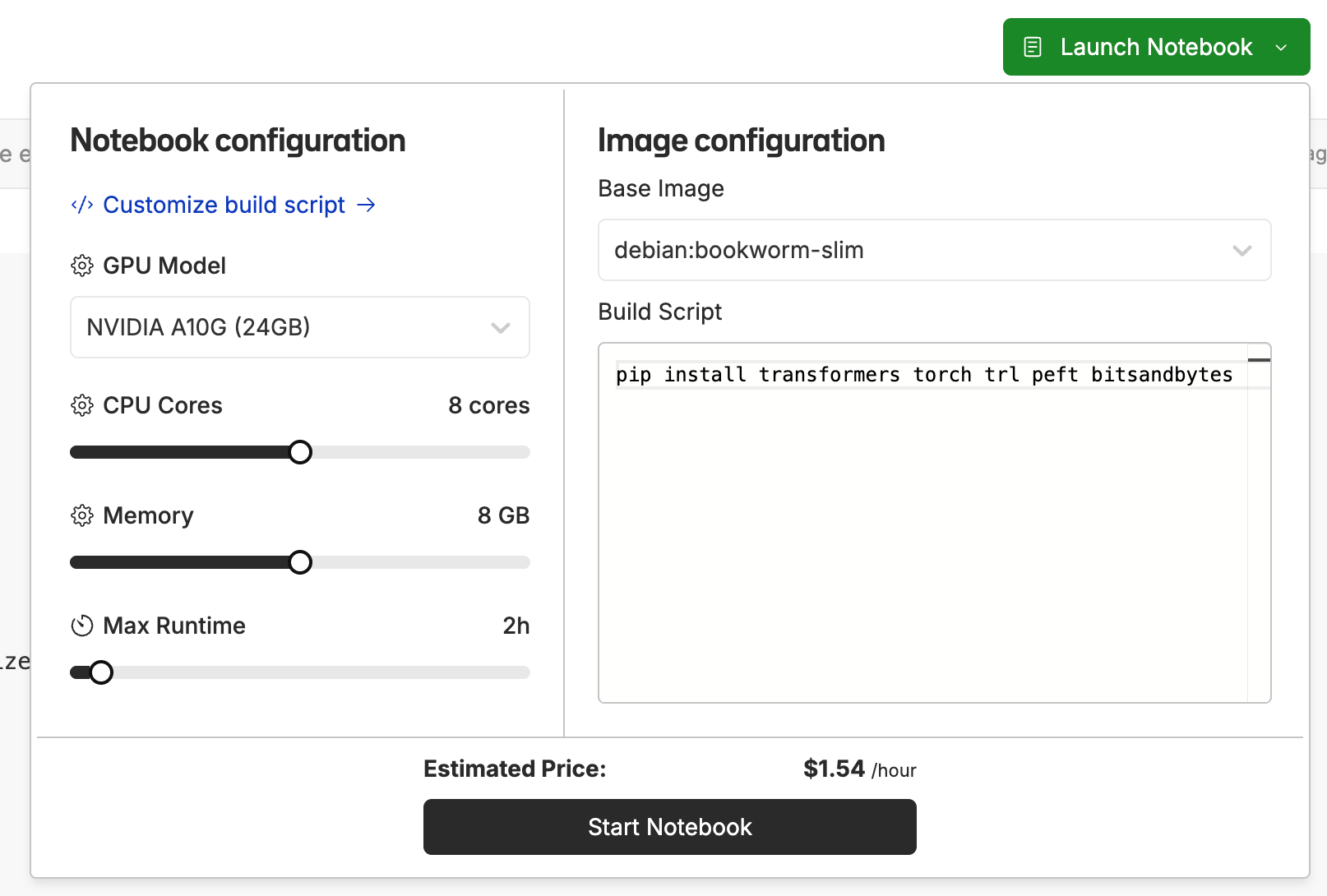
Make sure to configure your notebook with an A10G GPU and the following dependencies. Allocate at least 2 hours, 8 cpu cores and 8GB of memory for the training to complete in a reasonable amount of time.
```
pip install transformers torch trl peft bitsandbytes
```
 ### The Dataset
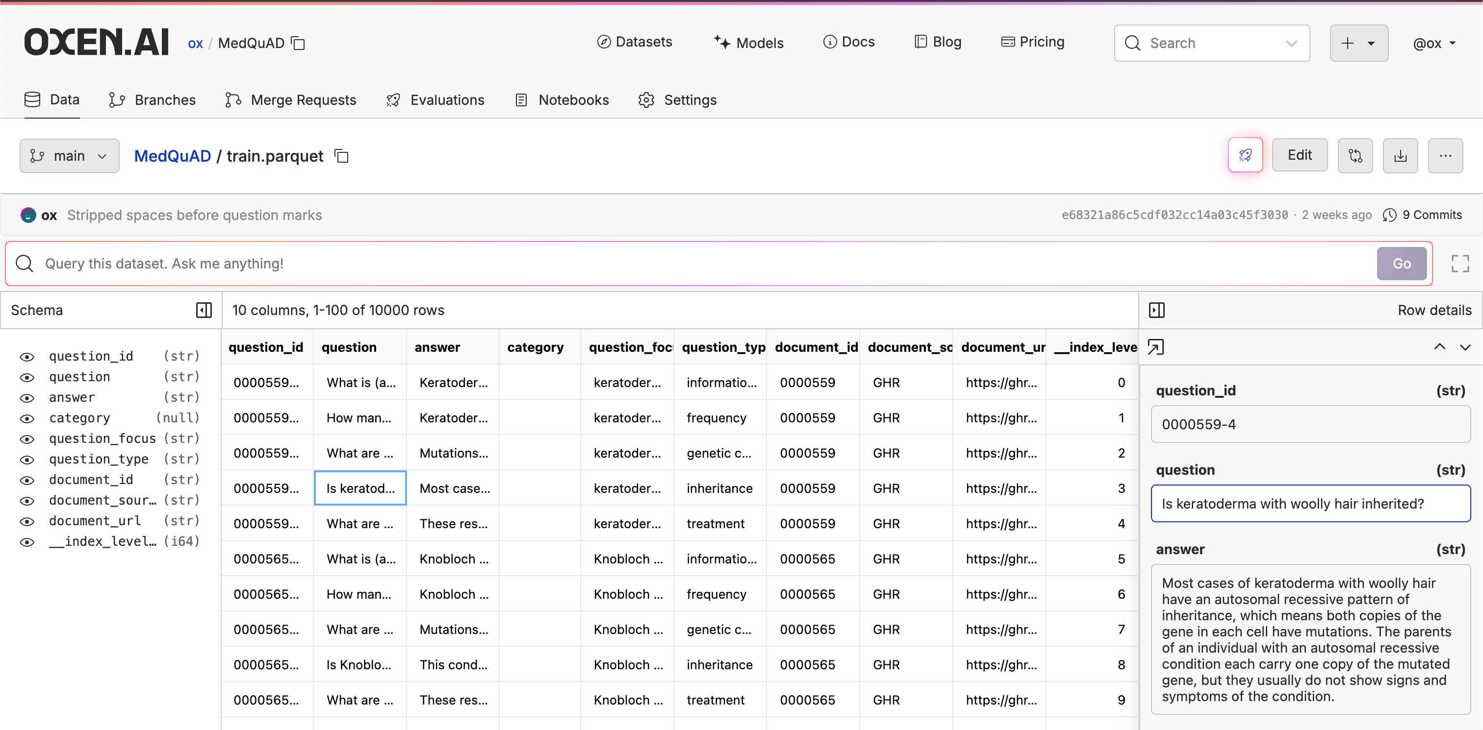
The dataset we will be using in this example is the [MedQuAD](https://www.oxen.ai/ox/MedQuAD/file/main/train.parquet) dataset. MedQuAD includes 47,457 medical question-answer pairs created from 12 NIH websites (e.g. cancer.gov, niddk.nih.gov, GARD, MedlinePlus Health Topics). The collection covers 37 question types (e.g. Treatment, Diagnosis, Side Effects) associated with diseases, drugs and other medical entities such as tests.
### The Dataset
The dataset we will be using in this example is the [MedQuAD](https://www.oxen.ai/ox/MedQuAD/file/main/train.parquet) dataset. MedQuAD includes 47,457 medical question-answer pairs created from 12 NIH websites (e.g. cancer.gov, niddk.nih.gov, GARD, MedlinePlus Health Topics). The collection covers 37 question types (e.g. Treatment, Diagnosis, Side Effects) associated with diseases, drugs and other medical entities such as tests.
 To load the dataset, we can use the `load_dataset` function from the `oxen.datasets` library. This is a wrapper around the Hugging Face [datasets](https://huggingface.co/docs/datasets/en/index) library, and is an easy way to load datasets from the Oxen.ai hub. To have fine-tuning work well, it is a good idea to have at least \~1000-10000 unique examples in your dataset. If you can collect more, that's even better.
Don't have a dataset yet? Checkout how to generate a [synthetic dataset](/examples/notebooks/generate_synthetic_datasets) from a stronger model to bootstrap your own.
```python theme={null}
from oxen.datasets import load_dataset
# Load dataset from the hub
raw_dataset = load_dataset("ox/MedQuAD", "train.parquet")
raw_dataset = raw_dataset.shuffle()
```
We then want to transform this dataset into a format that can be used for training a chatbot. This means mapping the question and answer pairs to a list of messages with roles. This is the format that most LLMs expect for training and inference.
```python theme={null}
system_message = """You are a highly trained medical doctor. Patients will ask you questions and you will provide and answer in plain english with easy to understand terms."""
def create_conversation(sample):
return {
"messages": [
{"role": "system", "content": system_message},
{"role": "user", "content": sample["question"]},
{"role": "assistant", "content": sample["answer"]}
]
}
# Convert dataset to OAI messages
dataset = raw_dataset.map(create_conversation, batched=False)
# Print formatted user prompt
print(json.dumps(dataset["train"][345]["messages"], indent=2))
```
### The Model
For this example, we will be using the [Qwen/Qwen2.5-1.5B-Instruct](https://huggingface.co/Qwen/Qwen2.5-1.5B-Instruct) model. This is a 1.5B parameter model that will be quick to train, and fast for inference. You can even download the weights and run on your laptop if you want.
To load the model, we can use the `AutoModelForCausalLM` and `AutoTokenizer` classes from the `transformers` library.
```python theme={null}
import torch
from transformers import AutoTokenizer, AutoModelForCausalLM, BitsAndBytesConfig, TextStreamer
model_name = "Qwen/Qwen2.5-1.5B-Instruct"
model = AutoModelForCausalLM.from_pretrained(
model_name,
torch_dtype="auto",
device_map="auto"
)
tokenizer = AutoTokenizer.from_pretrained(model_name)
```
Before you start training, it is a good idea to get a feel for the model. Start by writing a function to make a prediction given a prompt and system message.
```python theme={null}
def predict(tokenizer: AutoTokenizer, model: AutoModelForCausalLM, prompt: str):
system_prompt = "You are a medical professional who is helping a patient. Patients will ask you questions and you will answer them in plain English so that anyone can understand."
messages = [
{"role": "system", "content": system_prompt},
{"role": "user", "content": prompt}
]
text = tokenizer.apply_chat_template(
messages,
tokenize=False,
add_generation_prompt=True
)
model_inputs = tokenizer([text], return_tensors="pt").to(model.device)
streamer = TextStreamer(tokenizer)
generated_ids = model.generate(
**model_inputs,
max_new_tokens=1024,
streamer=streamer
)
generated_ids = [
output_ids[len(input_ids):] for input_ids, output_ids in zip(model_inputs.input_ids, generated_ids)
]
response = tokenizer.batch_decode(generated_ids, skip_special_tokens=True)[0]
return response
```
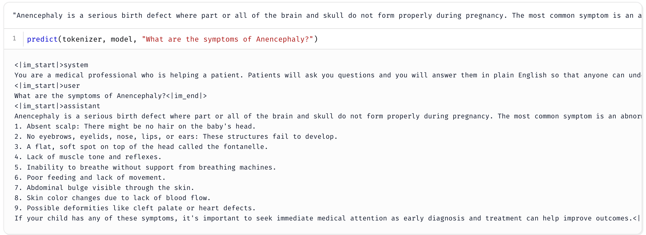
Call the `predict` function with a sample question.
```python theme={null}
predict(tokenizer, model, "What are the symptoms of Anencephaly?")
```
To load the dataset, we can use the `load_dataset` function from the `oxen.datasets` library. This is a wrapper around the Hugging Face [datasets](https://huggingface.co/docs/datasets/en/index) library, and is an easy way to load datasets from the Oxen.ai hub. To have fine-tuning work well, it is a good idea to have at least \~1000-10000 unique examples in your dataset. If you can collect more, that's even better.
Don't have a dataset yet? Checkout how to generate a [synthetic dataset](/examples/notebooks/generate_synthetic_datasets) from a stronger model to bootstrap your own.
```python theme={null}
from oxen.datasets import load_dataset
# Load dataset from the hub
raw_dataset = load_dataset("ox/MedQuAD", "train.parquet")
raw_dataset = raw_dataset.shuffle()
```
We then want to transform this dataset into a format that can be used for training a chatbot. This means mapping the question and answer pairs to a list of messages with roles. This is the format that most LLMs expect for training and inference.
```python theme={null}
system_message = """You are a highly trained medical doctor. Patients will ask you questions and you will provide and answer in plain english with easy to understand terms."""
def create_conversation(sample):
return {
"messages": [
{"role": "system", "content": system_message},
{"role": "user", "content": sample["question"]},
{"role": "assistant", "content": sample["answer"]}
]
}
# Convert dataset to OAI messages
dataset = raw_dataset.map(create_conversation, batched=False)
# Print formatted user prompt
print(json.dumps(dataset["train"][345]["messages"], indent=2))
```
### The Model
For this example, we will be using the [Qwen/Qwen2.5-1.5B-Instruct](https://huggingface.co/Qwen/Qwen2.5-1.5B-Instruct) model. This is a 1.5B parameter model that will be quick to train, and fast for inference. You can even download the weights and run on your laptop if you want.
To load the model, we can use the `AutoModelForCausalLM` and `AutoTokenizer` classes from the `transformers` library.
```python theme={null}
import torch
from transformers import AutoTokenizer, AutoModelForCausalLM, BitsAndBytesConfig, TextStreamer
model_name = "Qwen/Qwen2.5-1.5B-Instruct"
model = AutoModelForCausalLM.from_pretrained(
model_name,
torch_dtype="auto",
device_map="auto"
)
tokenizer = AutoTokenizer.from_pretrained(model_name)
```
Before you start training, it is a good idea to get a feel for the model. Start by writing a function to make a prediction given a prompt and system message.
```python theme={null}
def predict(tokenizer: AutoTokenizer, model: AutoModelForCausalLM, prompt: str):
system_prompt = "You are a medical professional who is helping a patient. Patients will ask you questions and you will answer them in plain English so that anyone can understand."
messages = [
{"role": "system", "content": system_prompt},
{"role": "user", "content": prompt}
]
text = tokenizer.apply_chat_template(
messages,
tokenize=False,
add_generation_prompt=True
)
model_inputs = tokenizer([text], return_tensors="pt").to(model.device)
streamer = TextStreamer(tokenizer)
generated_ids = model.generate(
**model_inputs,
max_new_tokens=1024,
streamer=streamer
)
generated_ids = [
output_ids[len(input_ids):] for input_ids, output_ids in zip(model_inputs.input_ids, generated_ids)
]
response = tokenizer.batch_decode(generated_ids, skip_special_tokens=True)[0]
return response
```
Call the `predict` function with a sample question.
```python theme={null}
predict(tokenizer, model, "What are the symptoms of Anencephaly?")
```
 Once you have predictions working from a model, it is good practice to have some sort of evaluation in place to see if fine-tuning actually improved the model. For situations where precision is important, you may want to build a [Human in the Loop](/examples/notebooks/eval_llm/human_in_the_loop) pipeline to evaluate the model's predictions. If you want to automate the evaluation process, you can use an [LLM as a Judge](/examples/notebooks/eval_llm/llm_as_a_judge) pipeline to evaluate the model's predictions.
To learn more about how to evaluate your model, check out Eugene Yan's [blog post](https://eugeneyan.com/writing/eval-process/) on fixing your evaluation process.
### Parameter Efficient Fine-Tuning
To make our fine-tuning process more efficient in terms of memory and time, we can use a technique called Parameter Efficient Fine-Tuning. This technique uses a technique called Low-Rank Adaptation (LoRA) to fine-tune the model. If you want to learn more about LoRA, check out the [LoRA paper](https://arxiv.org/abs/2106.09685) or our [Arxiv Dive](https://www.youtube.com/watch?v=_W85WtlfJcU) on the topic.
```python theme={null}
from peft import LoraConfig
# Define model init arguments
model_kwargs = dict(
attn_implementation="eager", # Use "flash_attention_2" when running on Ampere or newer GPU
torch_dtype=torch_dtype, # What torch dtype to use, defaults to auto
device_map="auto", # Let torch decide how to load the model
)
# BitsAndBytesConfig: Enables 4-bit quantization to reduce model size/memory usage
model_kwargs["quantization_config"] = BitsAndBytesConfig(
load_in_4bit=True,
bnb_4bit_use_double_quant=True,
bnb_4bit_quant_type='nf4',
bnb_4bit_compute_dtype=model_kwargs['torch_dtype'],
bnb_4bit_quant_storage=model_kwargs['torch_dtype'],
)
peft_config = LoraConfig(
lora_alpha=16,
lora_dropout=0.05,
r=16,
bias="none",
target_modules="all-linear",
task_type="CAUSAL_LM",
modules_to_save=["lm_head", "embed_tokens"] # make sure to save the lm_head and embed_tokens as you train the special tokens
)
```
This step is optional, but is good to know if you have limited resources. If you do not use parameter efficient fine-tuning, you will need to select a larger GPU for training.
### Branches for Experiments
It is rare that you will get a fine-tune perfect on the first try. You must have an experimental mindset and be willing to iterate. In this case we will be simply saving the trained models and results to new branches on the same repository. We will setup an `OxenExperiment` class that will handle creating a new branch, saving the model, and logging the results.
Branches are light weight in Oxen.ai, and by default will not be downloaded to your local machine when you do a clone. This means you can easily store model weights and other large assets on parallel branches and keep your `main` branch small and manageable.
```python theme={null}
from datetime import datetime
from pathlib import Path
import os
class OxenExperiment():
"""
An experiment helps log the experiment to an oxen repository,
keeps track of the name and creates a corresponding branch to save results to
"""
def __init__(self, repo, model_name, output_dir, experiment_type="SFT"):
self.repo = repo
self.output_dir = output_dir
# List the existing branches to figure out which experiment this is
branches = repo.branches()
experiment_number = 0
for branch in branches:
if branch.name.startswith(f"{experiment_type}_"):
experiment_number += 1
self.experiment_number = experiment_number
# Name the experiment with the experiment number and timestamp
short_model_name = model_name.split('/')[-1]
timestamp = datetime.now().strftime("%Y-%m-%d_%H-%M-%S")
self.name = f"{experiment_type}_{experiment_number}_{timestamp}_{short_model_name}"
# Set the output directory
self.dir = Path(os.path.join(self.output_dir, self.name))
# Create the output directory if it doesn't exist
os.makedirs(self.dir, exist_ok=True)
print(f"Creating experiment branch {self.name}")
repo.create_checkout_branch(self.name)
```
When you start a training run, you'll see a new branch in the repo with a prefix, number and a timestamp.
Once you have predictions working from a model, it is good practice to have some sort of evaluation in place to see if fine-tuning actually improved the model. For situations where precision is important, you may want to build a [Human in the Loop](/examples/notebooks/eval_llm/human_in_the_loop) pipeline to evaluate the model's predictions. If you want to automate the evaluation process, you can use an [LLM as a Judge](/examples/notebooks/eval_llm/llm_as_a_judge) pipeline to evaluate the model's predictions.
To learn more about how to evaluate your model, check out Eugene Yan's [blog post](https://eugeneyan.com/writing/eval-process/) on fixing your evaluation process.
### Parameter Efficient Fine-Tuning
To make our fine-tuning process more efficient in terms of memory and time, we can use a technique called Parameter Efficient Fine-Tuning. This technique uses a technique called Low-Rank Adaptation (LoRA) to fine-tune the model. If you want to learn more about LoRA, check out the [LoRA paper](https://arxiv.org/abs/2106.09685) or our [Arxiv Dive](https://www.youtube.com/watch?v=_W85WtlfJcU) on the topic.
```python theme={null}
from peft import LoraConfig
# Define model init arguments
model_kwargs = dict(
attn_implementation="eager", # Use "flash_attention_2" when running on Ampere or newer GPU
torch_dtype=torch_dtype, # What torch dtype to use, defaults to auto
device_map="auto", # Let torch decide how to load the model
)
# BitsAndBytesConfig: Enables 4-bit quantization to reduce model size/memory usage
model_kwargs["quantization_config"] = BitsAndBytesConfig(
load_in_4bit=True,
bnb_4bit_use_double_quant=True,
bnb_4bit_quant_type='nf4',
bnb_4bit_compute_dtype=model_kwargs['torch_dtype'],
bnb_4bit_quant_storage=model_kwargs['torch_dtype'],
)
peft_config = LoraConfig(
lora_alpha=16,
lora_dropout=0.05,
r=16,
bias="none",
target_modules="all-linear",
task_type="CAUSAL_LM",
modules_to_save=["lm_head", "embed_tokens"] # make sure to save the lm_head and embed_tokens as you train the special tokens
)
```
This step is optional, but is good to know if you have limited resources. If you do not use parameter efficient fine-tuning, you will need to select a larger GPU for training.
### Branches for Experiments
It is rare that you will get a fine-tune perfect on the first try. You must have an experimental mindset and be willing to iterate. In this case we will be simply saving the trained models and results to new branches on the same repository. We will setup an `OxenExperiment` class that will handle creating a new branch, saving the model, and logging the results.
Branches are light weight in Oxen.ai, and by default will not be downloaded to your local machine when you do a clone. This means you can easily store model weights and other large assets on parallel branches and keep your `main` branch small and manageable.
```python theme={null}
from datetime import datetime
from pathlib import Path
import os
class OxenExperiment():
"""
An experiment helps log the experiment to an oxen repository,
keeps track of the name and creates a corresponding branch to save results to
"""
def __init__(self, repo, model_name, output_dir, experiment_type="SFT"):
self.repo = repo
self.output_dir = output_dir
# List the existing branches to figure out which experiment this is
branches = repo.branches()
experiment_number = 0
for branch in branches:
if branch.name.startswith(f"{experiment_type}_"):
experiment_number += 1
self.experiment_number = experiment_number
# Name the experiment with the experiment number and timestamp
short_model_name = model_name.split('/')[-1]
timestamp = datetime.now().strftime("%Y-%m-%d_%H-%M-%S")
self.name = f"{experiment_type}_{experiment_number}_{timestamp}_{short_model_name}"
# Set the output directory
self.dir = Path(os.path.join(self.output_dir, self.name))
# Create the output directory if it doesn't exist
os.makedirs(self.dir, exist_ok=True)
print(f"Creating experiment branch {self.name}")
repo.create_checkout_branch(self.name)
```
When you start a training run, you'll see a new branch in the repo with a prefix, number and a timestamp.
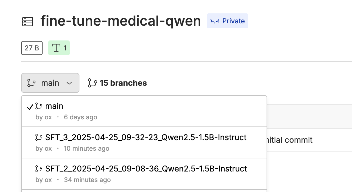 You can navigate to this branch and look in the `models` directory to see the model weights and other assets.
### Logging and Saving
Once we have the experiment setup, we will want to reference it during training and log our experiment results. To do this, we will setup an `OxenTrainerCallback` that will be called during training to save the model weights and our metrics. This is a subclass of the `TrainerCallback` class from the `transformers` library, which can be passed into our training loop.
```python theme={null}
from transformers import TrainerCallback
class OxenTrainerCallback(TrainerCallback):
def __init__(self, experiment: OxenExperiment, save_every):
self.experiment = experiment
self.save_every = save_every
self.log_file_name = "logs.jsonl"
self.log_file = os.path.join(self.experiment.dir, self.log_file_name)
self.dst_dir = os.path.dirname(self.log_file)
self.workspace = Workspace(
experiment.repo,
branch=f"{experiment.name}",
workspace_name=f"training_run_{experiment.experiment_number}"
)
self.df = DataFrame(
self.workspace,
self.log_file,
branch=f"{experiment.name}"
)
super().__init__()
def on_log(self, args, state, control, logs=None, **kwargs):
print("on_log.logs")
print(logs)
if "loss" in logs:
# add timestamp to logs
logs['timestamp'] = datetime.now().strftime("%Y-%m-%d %H:%M:%S")
# save logs to data frame
self.df.insert_row(logs)
def on_save(self, args, state, control, **kwargs):
print(f"on_save {state.global_step}")
if state.global_step % self.save_every == 0:
print(f"save every! {state.global_step} dir: {self.experiment.dir}")
# Save the checkpoints to model_dir/model_name/checkpoints/checkpoint_N
checkpoint_dir = os.path.join("checkpoints", f"checkpoint_{state.global_step}")
dst_dir = os.path.join(self.experiment.dir, checkpoint_dir)
self.workspace.add(self.experiment.dir, dst=dst_dir)
is_clean = self.workspace.status().is_clean()
print(f"Is Clean: {is_clean}")
if not self.workspace.status().is_clean():
self.workspace.commit(f"Saving model step {state.global_step}")
def on_step_end(self, args, state, control, **kwargs):
print(f"on_step_end {state.global_step}")
```
Since we are subclassing the `TrainerCallback` class, we implement the `on_save` and `on_log` methods. The `on_save` method is called when the model is saved to disk, and the `on_log` method is called when the model is trained on a batch, reporting loss and other useful metrics.
The most important concepts here are the `Workspace` and `DataFrame` objects from the `oxenai` library. The `Workspace` is a wrapper around the branch that we are currently on. This allows us to write data to the remote branch without committing the changes to the branch. Think of it like your local repo of unstaged changes, but for remote branches. To navigate to your workspaces, use the branch dropdown and then look at the active workspaces for a file.
You can navigate to this branch and look in the `models` directory to see the model weights and other assets.
### Logging and Saving
Once we have the experiment setup, we will want to reference it during training and log our experiment results. To do this, we will setup an `OxenTrainerCallback` that will be called during training to save the model weights and our metrics. This is a subclass of the `TrainerCallback` class from the `transformers` library, which can be passed into our training loop.
```python theme={null}
from transformers import TrainerCallback
class OxenTrainerCallback(TrainerCallback):
def __init__(self, experiment: OxenExperiment, save_every):
self.experiment = experiment
self.save_every = save_every
self.log_file_name = "logs.jsonl"
self.log_file = os.path.join(self.experiment.dir, self.log_file_name)
self.dst_dir = os.path.dirname(self.log_file)
self.workspace = Workspace(
experiment.repo,
branch=f"{experiment.name}",
workspace_name=f"training_run_{experiment.experiment_number}"
)
self.df = DataFrame(
self.workspace,
self.log_file,
branch=f"{experiment.name}"
)
super().__init__()
def on_log(self, args, state, control, logs=None, **kwargs):
print("on_log.logs")
print(logs)
if "loss" in logs:
# add timestamp to logs
logs['timestamp'] = datetime.now().strftime("%Y-%m-%d %H:%M:%S")
# save logs to data frame
self.df.insert_row(logs)
def on_save(self, args, state, control, **kwargs):
print(f"on_save {state.global_step}")
if state.global_step % self.save_every == 0:
print(f"save every! {state.global_step} dir: {self.experiment.dir}")
# Save the checkpoints to model_dir/model_name/checkpoints/checkpoint_N
checkpoint_dir = os.path.join("checkpoints", f"checkpoint_{state.global_step}")
dst_dir = os.path.join(self.experiment.dir, checkpoint_dir)
self.workspace.add(self.experiment.dir, dst=dst_dir)
is_clean = self.workspace.status().is_clean()
print(f"Is Clean: {is_clean}")
if not self.workspace.status().is_clean():
self.workspace.commit(f"Saving model step {state.global_step}")
def on_step_end(self, args, state, control, **kwargs):
print(f"on_step_end {state.global_step}")
```
Since we are subclassing the `TrainerCallback` class, we implement the `on_save` and `on_log` methods. The `on_save` method is called when the model is saved to disk, and the `on_log` method is called when the model is trained on a batch, reporting loss and other useful metrics.
The most important concepts here are the `Workspace` and `DataFrame` objects from the `oxenai` library. The `Workspace` is a wrapper around the branch that we are currently on. This allows us to write data to the remote branch without committing the changes to the branch. Think of it like your local repo of unstaged changes, but for remote branches. To navigate to your workspaces, use the branch dropdown and then look at the active workspaces for a file.
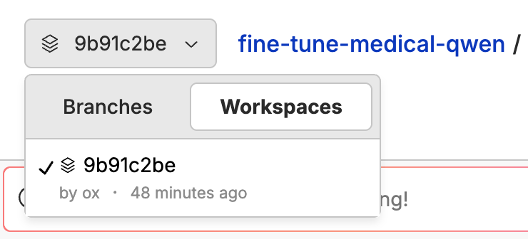 During training it would be expensive to commit the changes to the branch every step, so instead we use a `Workspace` to write the temporary results, and then can commit the changes to the branch after training is complete.
```python theme={null}
from oxen import Workspace, DataFrame
self.workspace = Workspace(
experiment.repo,
branch=f"{experiment.name}",
workspace_name=f"training_run_{experiment.experiment_number}"
)
self.df = DataFrame(
self.workspace,
self.log_file,
branch=f"{experiment.name}"
)
```
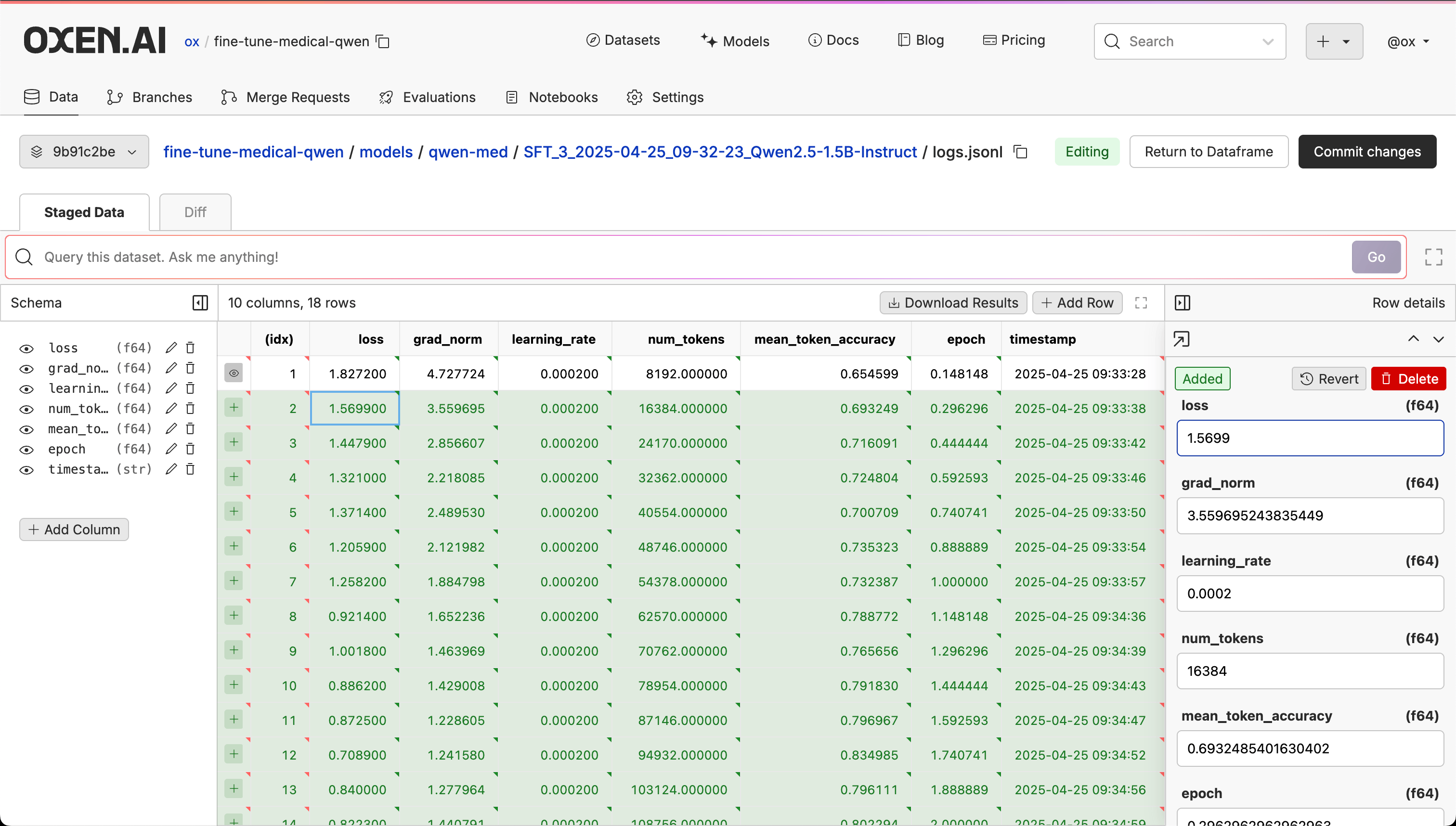
The DataFrame allows us to write rows and columns to the log file. We can read from this to make plots and analyze the results. When clicking on a data frame's workspace, you can see a preview of the data that is written during the `on_log` method.
```python theme={null}
def on_log(self, args, state, control, logs=None, **kwargs):
# add timestamp to logs
logs['timestamp'] = datetime.now().strftime("%Y-%m-%d %H:%M:%S")
# save logs to data frame
self.df.insert_row(logs)
```
During training it would be expensive to commit the changes to the branch every step, so instead we use a `Workspace` to write the temporary results, and then can commit the changes to the branch after training is complete.
```python theme={null}
from oxen import Workspace, DataFrame
self.workspace = Workspace(
experiment.repo,
branch=f"{experiment.name}",
workspace_name=f"training_run_{experiment.experiment_number}"
)
self.df = DataFrame(
self.workspace,
self.log_file,
branch=f"{experiment.name}"
)
```
The DataFrame allows us to write rows and columns to the log file. We can read from this to make plots and analyze the results. When clicking on a data frame's workspace, you can see a preview of the data that is written during the `on_log` method.
```python theme={null}
def on_log(self, args, state, control, logs=None, **kwargs):
# add timestamp to logs
logs['timestamp'] = datetime.now().strftime("%Y-%m-%d %H:%M:%S")
# save logs to data frame
self.df.insert_row(logs)
```
 With all the building blocks in place, we can then chain all of these classes together and specify the `RemoteRepo`, model name, and output directory.
```python theme={null}
from oxen import RemoteRepo
output_dir = "models/qwen-med"
repo = RemoteRepo("ox/fine-tune-medical-qwen")
experiment = OxenExperiment(repo, model_name, output_dir)
trainer_callback = OxenTrainerCallback(experiment)
```
### The Training Loop
The `trl` library from Hugging Face is an easy to use library for training and fine-tuning models. We can use the `SFTConfig` class to setup our training loop. This determines our batch size, learning rate, number of epochs, and other hyperparameters.
```python theme={null}
from trl import SFTConfig
logging_steps = 1
args = SFTConfig(
output_dir=experiment.dir, # directory to save and repository id
num_train_epochs=1, # number of training epochs
per_device_train_batch_size=1, # batch size per device during training
gradient_accumulation_steps=4, # number of steps before performing a backward/update pass
gradient_checkpointing=True, # use gradient checkpointing to save memory
optim="adamw_torch_fused", # use fused adamw optimizer
logging_steps=logging_steps, # log every N steps
save_strategy="epoch", # save the weights the end of an epoch
learning_rate=2e-4, # learning rate, based on QLoRA paper
fp16=True if torch_dtype == torch.float16 else False, # use float16 precision
bf16=True if torch_dtype == torch.bfloat16 else False, # use bfloat16 precision
max_grad_norm=0.3, # max gradient norm based on QLoRA paper
warmup_ratio=0.03, # warmup ratio based on QLoRA paper
lr_scheduler_type="constant", # use constant learning rate scheduler
)
```
Once you have set up the training arguments, you can then setup the training loop. Pass in the model, training arguments, peft config, the training dataset, and callbacks.
```python theme={null}
from trl import SFTTrainer
# Create Trainer object
trainer = SFTTrainer(
model=model,
args=args,
train_dataset=dataset["train"],
peft_config=peft_config,
processing_class=tokenizer,
callbacks=[OxenTrainerCallback(experiment)]
)
```
Finally, you can then train the model.
```python theme={null}
trainer.train()
```
This should take just under 2 hours with the settings above. Once the training is complete, you will be able to download the model weights from the experiment branch and use them for inference.
### Evaluation
Just because the fine-tune has completed, does not mean your job is done. Now you must evaluate the model to see if it is any good. With the dataset that we have been using, it is hard to do an exact string match evaluation on outputs to tell if the fine-tuned model is better than the original.
Instead, we will use an [LLM as a Judge](/examples/notebooks/eval_llm/llm_as_a_judge) pipeline to evaluate the model's predictions. This will allow us to quickly see if the fine-tuned model is better than the original.
With all the building blocks in place, we can then chain all of these classes together and specify the `RemoteRepo`, model name, and output directory.
```python theme={null}
from oxen import RemoteRepo
output_dir = "models/qwen-med"
repo = RemoteRepo("ox/fine-tune-medical-qwen")
experiment = OxenExperiment(repo, model_name, output_dir)
trainer_callback = OxenTrainerCallback(experiment)
```
### The Training Loop
The `trl` library from Hugging Face is an easy to use library for training and fine-tuning models. We can use the `SFTConfig` class to setup our training loop. This determines our batch size, learning rate, number of epochs, and other hyperparameters.
```python theme={null}
from trl import SFTConfig
logging_steps = 1
args = SFTConfig(
output_dir=experiment.dir, # directory to save and repository id
num_train_epochs=1, # number of training epochs
per_device_train_batch_size=1, # batch size per device during training
gradient_accumulation_steps=4, # number of steps before performing a backward/update pass
gradient_checkpointing=True, # use gradient checkpointing to save memory
optim="adamw_torch_fused", # use fused adamw optimizer
logging_steps=logging_steps, # log every N steps
save_strategy="epoch", # save the weights the end of an epoch
learning_rate=2e-4, # learning rate, based on QLoRA paper
fp16=True if torch_dtype == torch.float16 else False, # use float16 precision
bf16=True if torch_dtype == torch.bfloat16 else False, # use bfloat16 precision
max_grad_norm=0.3, # max gradient norm based on QLoRA paper
warmup_ratio=0.03, # warmup ratio based on QLoRA paper
lr_scheduler_type="constant", # use constant learning rate scheduler
)
```
Once you have set up the training arguments, you can then setup the training loop. Pass in the model, training arguments, peft config, the training dataset, and callbacks.
```python theme={null}
from trl import SFTTrainer
# Create Trainer object
trainer = SFTTrainer(
model=model,
args=args,
train_dataset=dataset["train"],
peft_config=peft_config,
processing_class=tokenizer,
callbacks=[OxenTrainerCallback(experiment)]
)
```
Finally, you can then train the model.
```python theme={null}
trainer.train()
```
This should take just under 2 hours with the settings above. Once the training is complete, you will be able to download the model weights from the experiment branch and use them for inference.
### Evaluation
Just because the fine-tune has completed, does not mean your job is done. Now you must evaluate the model to see if it is any good. With the dataset that we have been using, it is hard to do an exact string match evaluation on outputs to tell if the fine-tuned model is better than the original.
Instead, we will use an [LLM as a Judge](/examples/notebooks/eval_llm/llm_as_a_judge) pipeline to evaluate the model's predictions. This will allow us to quickly see if the fine-tuned model is better than the original.